While hidecan was designed with the goal of representing GWAS and DE results with lists of candidate genes, in principle it can be used to visualise any genomic feature that can be mapped to a physical location on the genome; for example significant methylation sites, transposable elements location, chromatin accessibility data etc. To facilitate this, it is possible to add one or more custom data types into a hidecan plot.
Adding one custom data type – genomic locations
Let us start by simulating a new set of results – for simplicity we’ll assume that we have results from a DNA methylation study on the same markers that were used for the GWAS analysis:
x <- get_example_data()

set.seed(586)
x$METH <- x$GWAS |>
  ## shuffling the scores around to get different "significant" markers
  mutate(score = sample(score, n(), replace = FALSE))
We can add this new data to the hidecan plot through the
custom_list argument of the hidecan_plot()
function (we’ll only look at two chromosomes for simplicity), and use
the score_thr_custom argument to set the significance
threshold on the score:
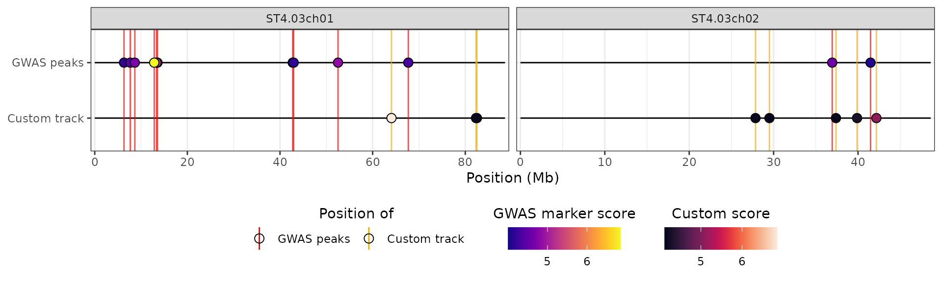
hidecan_plot(
  gwas_list = x[["GWAS"]],
  score_thr_gwas = -log10(0.0001),
  chroms = c("ST4.03ch01", "ST4.03ch02"),
  custom_list = x[["METH"]],
  score_thr_custom = -log10(0.0001)
)
Importantly, the data-frame that is passed to
custom_list must contain at least the following columns:
chromosome, position OR start and
end, and score. If you provide a table with
start and end columns but no
position column, it will be computed as the mid-point
between the start and end of the features.
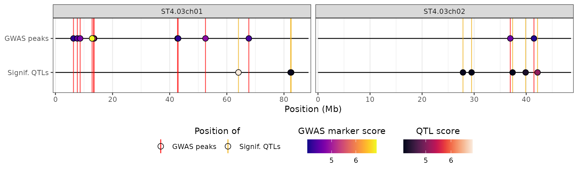
We can customise the labels and colours used for this custom track
with the help of the hidecan_aes() function:
plot_aes <- hidecan_aes()

str(plot_aes, max.level = 1)
#> List of 5
#>  $ QTL_data_thr   :List of 7
#>  $ GWAS_data_thr  :List of 7
#>  $ DE_data_thr    :List of 7
#>  $ CAN_data_thr   :List of 7
#>  $ CUSTOM_data_thr:List of 7

plot_aes[["CUSTOM_data_thr"]]
#> $y_label
#> [1] "Custom track"
#>
#> $show_as_rect
#> [1] FALSE
#>
#> $line_colour
#> [1] "darkgoldenrod2"
#>
#> $point_shape
#> [1] 21
#>
#> $show_name
#> [1] FALSE
#>
#> $fill_scale
#> <ScaleContinuous>
#>  Range:
#>  Limits:    0 --    1
#>
#> $rect_width
#> [1] 0.5
In particular, we will change the name given to the track, as well as the name used for the legend:
plot_aes$CUSTOM_data_thr$y_label <- "Signif. methylation sites"

plot_aes$CUSTOM_data_thr$fill_scale$name <- "Methylation score"

# We could also change the entire legend with:

# default_aes$CUSTOM_data_thr$fill_scale <- scale_fill_viridis(
#   "Methylation score",
#   option = "inferno",
#   guide = guide_colourbar(
#     title.position = "top",
#     title.hjust = 0.5,
#     order = 5 # ensures this legend is shown after the one for GWAS scores
#   )
# )
We will use these values in the hidecan plot by passing the list
through the custom_aes argument:
hidecan_plot(
  gwas_list = x[["GWAS"]],
  score_thr_gwas = -log10(0.0001),
  chroms = c("ST4.03ch01", "ST4.03ch02"),
  custom_list = x[["METH"]],
  score_thr_custom = -log10(0.0001),
  custom_aes = plot_aes
)
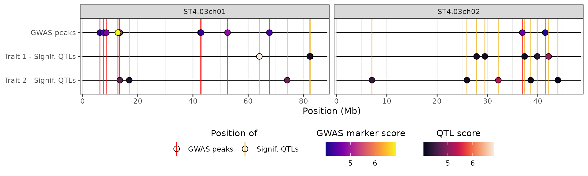
Note that, as for the other supported data types, we can pass more
than one data-frame to custom_list to get several tracks of
methylated sites:
## Simulating a second set of methylation data
set.seed(779)
x$METH2 <- x$METH |>
  mutate(score = sample(score, n(), replace = FALSE))

hidecan_plot(
  gwas_list = x[["GWAS"]],
  score_thr_gwas = -log10(0.0001),
  score_thr_de = -log10(0.05),
  log2fc_thr = 0,
  chroms = c("ST4.03ch01", "ST4.03ch02"),
  custom_list = list("Condition 1" = x[["METH"]],
                     "Condition 2" = x[["METH2"]]),
  score_thr_custom = -log10(0.0001),
  custom_aes = plot_aes
)
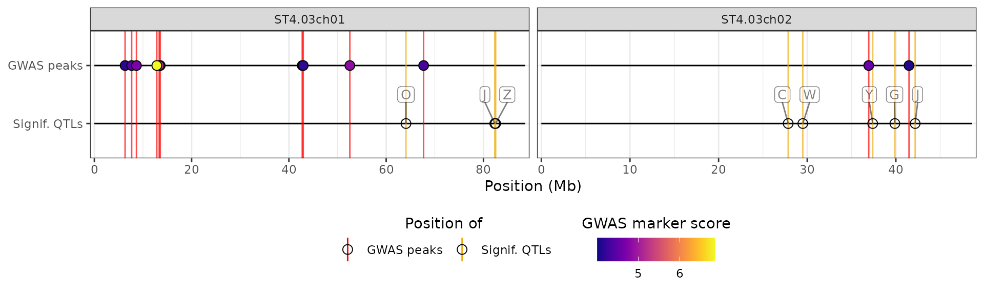
By default, the values in the score column are shown as
the points colour, but we can hide it by setting the
fill_scale element of our aesthetics list to
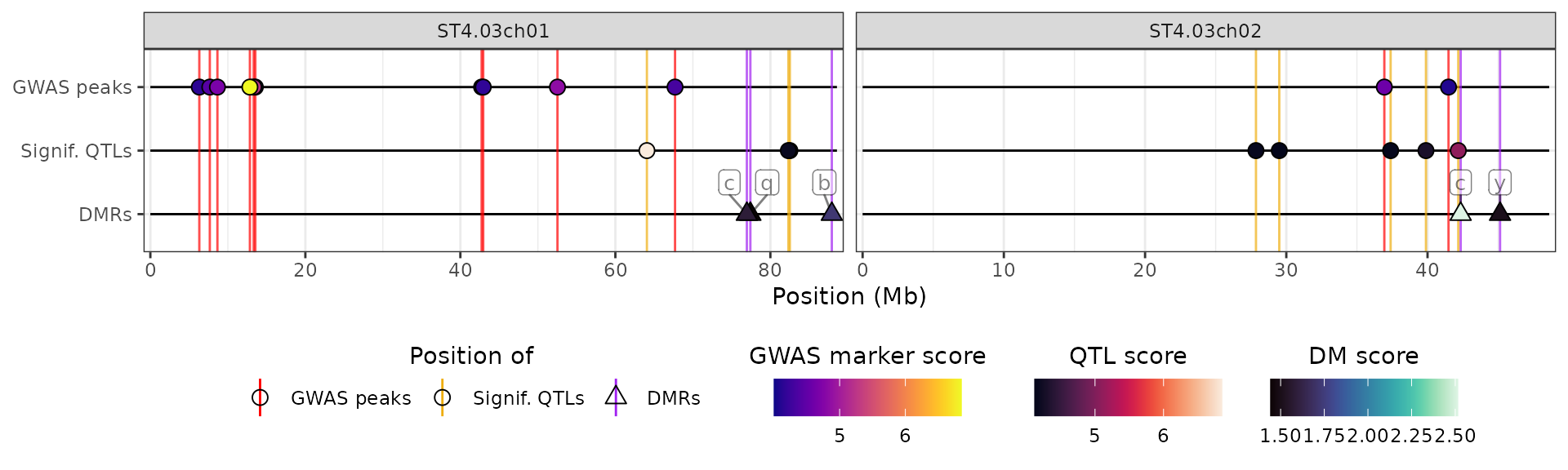
NULL. Also, we can add labels to the significant points, by
adding a name column to the data-frame, and setting the
show_name element of our aesthetics list to
TRUE:
## Creating fake names for the markers
set.seed(342)
x$METH <- x$METH |>
  mutate(name = sample(LETTERS, n(), replace = TRUE))

plot_aes2 <- plot_aes

plot_aes2$CUSTOM_data_thr$show_name <- TRUE
plot_aes2$CUSTOM_data_thr$fill_scale <- NULL

hidecan_plot(
  gwas_list = x[["GWAS"]],
  score_thr_gwas = -log10(0.0001),
  chroms = c("ST4.03ch01", "ST4.03ch02"),
  custom_list = x[["METH"]],
  score_thr_custom = -log10(0.0001),
  custom_aes = plot_aes2
)
Adding one custom data type – genomic regions
We can also add a track showcasing genomic regions, i.e. similar to QTL regions. As an example, let’s say that we have a list of regions with low chromatin accessibility:
x$CHA <- tibble(
  chromosome = c("ST4.03ch01", "ST4.03ch01", "ST4.03ch02"),
  start = c(25e6, 60e6, 5e6),
  end = c(29e6, 62e6, 12e6),
  score = c(6.3, 4.5, 5.2)
)
We need to specify that these should be represented using rectangles
spanning the length of the regions, rather than as points (as for GWAS
or DE results). This is done via the show_as_rect argument
in the aesthetics list:
plot_aes_cha <- hidecan_aes()

plot_aes_cha$CUSTOM_data_thr$show_as_rect <- TRUE

## Customising other aspects of the new track
plot_aes_cha$CUSTOM_data_thr$y_label <- "Low chromatin acc."
plot_aes_cha$CUSTOM_data_thr$fill_scale$name <- "Accessibility score"
plot_aes_cha$CUSTOM_data_thr$line_colour <- "firebrick"

hidecan_plot(
  gwas_list = x[["GWAS"]],
  score_thr_gwas = -log10(0.0001),
  chroms = c("ST4.03ch01", "ST4.03ch02"),
  custom_list = x[["CHA"]],
  score_thr_custom = -log10(0.0001),
  custom_aes = plot_aes_cha
)
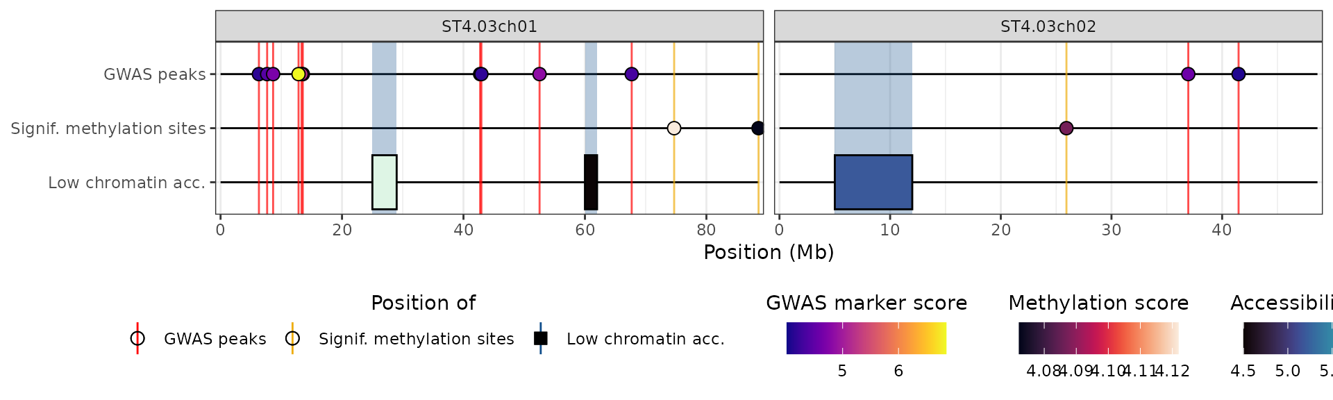
Adding several custom data types
It is also possible to add more than one custom data type. For example, let’s combine our methylated bases and our low accessibility regions into one plot.
Importantly, the significance threshold encoded by the
score_thr_custom argument of hidecan_plot()
will be used for all custom datasets, so if we don’t want to use the
same significance threshold on our methylation and chromatin
accessibility data, we need to perform the filtering of significant
features by hand before and then set the threshold to 0:
The key to specifying that the two custom datasets are different data
types is to add to the new data-frame an argument called
aes_type, which is simply a label that tells the function
which aesthetics settings it should use from the list passsed to
custom_aes. We will retain the aesthetics we have set for
the QTL scores, and create new aesthetics for the methylation data:
## Adding the aes_type attribute to the methylation data
attr(x$CHA, "aes_type") <- "CHA"

## The name of the new element in the aesthetics list must match the value of
## the aes_type attribute
plot_aes$CHA <- list(
  y_label = "Low chromatin acc.",
  show_as_rect = TRUE,
  line_colour = "dodgerblue4",
  point_shape = 24, ## this doesn't matter as we are representing regions
  show_name = FALSE,
  fill_scale = scale_fill_viridis(
    "Accessibility score",
    option = "mako",
    guide = guide_colourbar(
      title.position = "top",
      title.hjust = 0.5,
      order = 5
    )
  ),
  rect_width = 0.5
)

hidecan_plot(
  gwas_list = x[["GWAS"]],
  score_thr_gwas = -log10(0.0001),
  chroms = c("ST4.03ch01", "ST4.03ch02"),
  custom_list = list(x[["METH"]], x[["CHA"]]),
  score_thr_custom = 0, ## no filtering, has been done manually
  custom_aes = plot_aes
)
There are no restrictions on the number of custom data types that can be added to a hidecan plot.